- Introducing A Matrix A With Elements A G X And Vectors C C C Cn And Y Y 2 The Superscript Denotes Tra 1 (98.09 KiB) Viewed 34 times
- Introducing A Matrix A With Elements A G X And Vectors C C C Cn And Y Y 2 The Superscript Denotes Tra 2 (98.45 KiB) Viewed 34 times
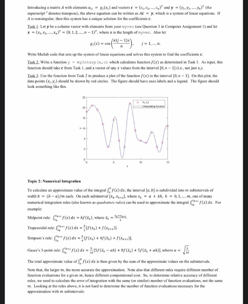
Introducing a matrix A with elements a = g(x) and vectors c = (C₁, C₂, Cn) and y = (y₁.2.₁) (the superscript denotes transpose), the above equation can be written as Ac = y, which is a system of linear equations. If A is nonsingular, then this system has a unique solution for the coefficients c. Task 1: Let y be a column vector with elements from your myvec (see Question 3 in Computer Assignment 1) and let x = (x₁,x₂,...,x₁) = (0,1,2,..., n-1)", where n is the length of myvec. Also let (n(j-1)x) g(x) = cos j = 1,..., n. n Write Matlab code that sets up the system of linear equations and solves this system to find the coefficients c. Task 2: Write a function y = myInterp (x, c) which calculates function f(x) as determined in Task 1. As input, this function should take c from Task 1, and a vector of any x values from the interval [0, n - 1] (i.c., not just x₁). Task 3: Use the function from Task 2 to produce a plot of the function f(x) in the interval [0, n-1]. On this plot, the data points (x,y) should be shown by red circles. The figure should have axes labels and a legend. The figure should look something like this 25 0 (x,y) Interpolating function 20 15 > 10 5 -5 10 15 Topic 2: Numerical Integration To calculate an approximate value of the integral f f(x) dx, the interval [a, b] is subdivided into m subintervals of width h= (b-a)/m each. On each subinterval [XX+1], where x = a + kh, k = 0, 1,..., m, one of many numerical integration rules (also known as quadrature rules) can be used to approximate the integral f***¹ f(x) dx. For example: Midpoint rule: + f(x) dx hf (x), where ** =******1 Trapezoidal rule: f**+ f(x) dx = [f(xx) + f(xx+1)]. Simpson's rule: ***¹ f(x) dx = [f(x) + 4f(xx) + f(xx+1)]. Gauss's 3-point rule: ***¹ f(x) dx = [5f(xx-ah) +8f(x) +5f (x + ah)], where a = The total approximate value of f f(x) dx is then given by the sum of the approximate values on the subintervals. Note that, the larger m, the more accurate the approximation. Note also that different rules require different number of function evaluations for a given m, hence different computational cost. So, to determine relative accuracy of different rules, we need to calculate the error of integration with the same (or similar) number of function evaluations, not the same m. Looking at the rules above, it is not hard to determine the number of function evaluations necessary for the approximation with m subintervals: 0
Midpoint rule: Nf = m; Trapezoidal rule: N₁ = m + 1; Simpson's rule: Nf = 2m + 1; Gauss's 3-point rule: N = 3m. Task 4: Calculate approximate value of the integral f-1 f(x) dx, where f(x) is the function defined in Task 2. Obtain results for each of the four rules above with Nf = 33. Try to write your code in such a way that it uses not more than Nf evaluations of function f(x). -19, (x), with n = Note: If you were not able to obtain correct function f(x) in Task 2, then use the function f(x) = 10 and g, (x) as defined above. Task 5: Determine the magnitude of the error (i.e., the difference between the approximate and the exact value) of each of the four approximate results from Task 4. To do this, you need to find the exact value of the integral, which you can calculate analytically and then evaluate the obtained formula in Matlab. Task 6: For each of the four rules, determine the smallest number N, such that the magnitude of the error is smaller than 10-8. Explain how you determined the required value of Nf. Task 7: Study the literature on numerical integration and implement a quadrature rule of your choice. You should aim to find a rule which will give the smallest possible error for a given number of function evaluations. Discuss whether this rule is more or less accurate than the four rules presented above.