Answer Happy

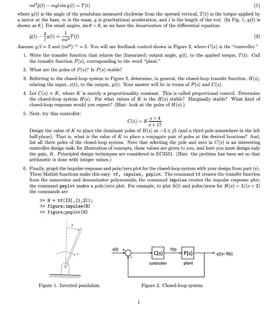
Vt) - x) = PT() ml?j(t) - mgl sin y(t) = T(t) (1) where y(t) is the angle of the pendulum measured clockwise from the upward vertical, T(t) is the torque applied by a motor at the base, m is the mass, g is gravitational acceleration, and l is the length of the rod. (In Fig. 1, y(t) is shown as 6.) For small angles, sin 0 = 0, so we have the linearization of the differential equation: (2) Assume g/l = 2 and (m12)-1 = 2. You will use feedback control shown in Figure 2, where C(s) is the "controller." 1. Write the transfer function that relates the linearized) output angle, y(t), to the applied torque, T(t). Call the transfer function P(s), corresponding to the word “plant." 2. What are the poles of P(s)? Is P(s) stable? 3. Referring to the closed-loop system in Figure 2, determine, in general, the closed-loop transfer function, H(s), relating the input, z(t), to the output, y(t). Your answer will be in terms of P(s) and C(s). 4. Let C(s) = K, where K is merely a proportionality constant. This is called proportional control. Determine the closed-loop system H(s). For what values of K is the H(s) stable? Marginally stable? What kind of closed-loop response would you expect? (Hint: look at the poles of H(s).) 5. Next, try this controller: C(s) = K 8+4 8 + 17 Design the value of K to place the dominant poles of H() at -3 j5 (and a third pole somewhere in the left half-plane). That is, what is the value of K to place a conjugate pair of poles at the desired locations? And, list all three poles of the closed-loop system. Note that selecting the pole and zero in C($) is an interesting controller design task; for illustration of concepts, these values are given to you, and here you must design only the gain, K. Principled design techniques are considered in EC3551. (Hint: the problem has been set so that arithmetic is done with integer values.) 6. Finally, graph the impulse response and pole/zero plot for the closed-loop system with your design from part (e). Three Matlab functions make this easy: tf, impulse, pzplot. The command tf creates the transfer function from the numerator and denominator polynomials; the command impulse creates the impulse response plot; the command pzplot makes a pole/zero plot. For example, to plot h(t) and poles/zeros for H(s) = 3/(x + 2) the commands are >> H = tf([3],[1,2]); >> figure; impulse (H) >> figure;pzplot(H) x(t) T(t) C(s) P(s) y(t)= 0(t) controller plant Figure 1. Inverted pendulum Figure 2. Closed-loop system 1