Answer Happy

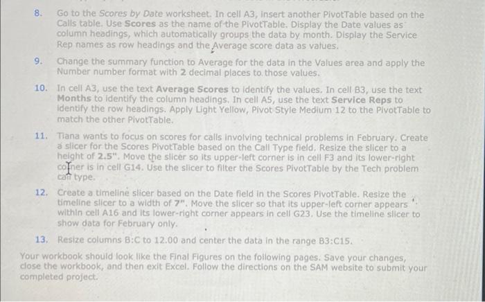
8. Go to the Scores by Date worksheet. In cell A3, Insert another Pivot Table based on the Calls table. Use Scores as the name of the Pivottable. Display the Date values as column headings, which automatically groups the data by month. Display the Service Rep names as row headings and the Average score data as values. 9. Change the summary function to Average for the data in the Values area and apply the Number number format with 2 decimal places to those values. 10. In cell A3, use the text Average Scores to identify the values. In cell B3, use the text Months to identify the column headings, In cell AS, use the text Service Reps to Identify the row headings. Apply Light Yellow, Pivot Style Medium 12 to the pivotTable to match the other Pivottable. 11. Tiana wants to focus on scores for calls involving technical problems in February. Create a slicer for the Scores PlvotTable based on the Call Type field, Resize the slicer to a height of 2.5". Move the slicer so its upper-left corner is in cell F3 and its lower right Ther is in cell G14. Use the slicer to filter the Scores PivotTable by the Tech problem can type 12. Create a timeline Slicer based on the Date field in the Scores PivotTable. Resize the timeline slicer to a width of 7". Move the slicer so that its upper-left corner appears within cell A16 and its lower-right corner appears in cell G23. Use the timeline sicer to show data for February only 13. Resize columns B:C to 12.00 and center the data in the range B3:015. Your workbook should look like the Final Figures on the following pages. Save your changes, close the workbook, and then exit Excel. Follow the directions on the SAM website to submit your completed project.