Answer Happy

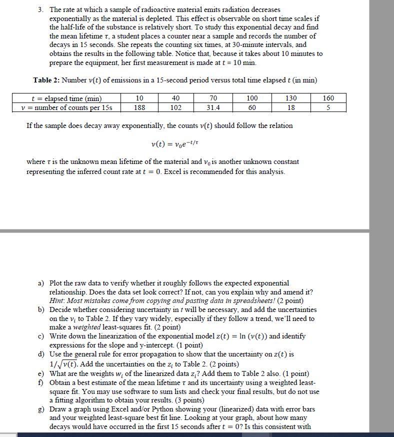
3. The rate at which a sample of radioactive material emits radiation decreases exponentially as the material is depleted. This effect is observable on short time scales if the half-life of the substance is relatively short. To study this exponential decay and find the mean lifetime T, a student places a counter near a sample and records the number of decays in 15 seconds. She repeats the counting six times, at 30-minute intervals, and obtains the results in the following table. Notice that, because it takes about 10 minutes to prepare the equipment, her first measurement is made at t = 10 min. Table 2: Number v(t) of emissions in a 15-second period versus total time elapsed t (in min) t = elapsed time (min) v = number of counts per 15s If the sample does decay away exponentially, the counts v(t) should follow the relation v(t) = voe-t/t where t is the unknown mean lifetime of the material and vois another unknown constant representing the inferred count rate at t = 0. Excel is recommended for this analysis. 10 188 40 102 70 31.4 100 60 130 18 a) Plot the raw data to verify whether it roughly follows the expected exponential relationship. Does the data set look correct? If not, can you explain why and amend it? Hint: Most mistakes come from copying and pasting data in spreadsheets! (2 point) b) Decide whether considering uncertainty in t will be necessary, and add the uncertainties on the v; to Table 2. If they vary widely, especially if they follow a trend, we'll need to make a weighted least-squares fit. (2 point) c) Write down the linearization of the exponential model z(t) = ln (v(t)) and identify expressions for the slope and y-intercept. (1 point) d) Use the general rule for error propagation to show that the uncertainty on z(t) is 1/√v(t). Add the uncertainties on the z; to Table 2. (2 points) e) What are the weights w of the linearized data z;? Add them to Table 2 also. (1 point) f) Obtain a best estimate of the mean lifetime 7 and its uncertainty using a weighted least- square fit. You may use software to sum lists and check your final results, but do not use a fitting algorithm to obtain your results. (3 points) g) Draw a graph using Excel and/or Python showing your (linearized) data with error bars and your weighted least-square best fit line. Looking at your graph, about how many decays would have occurred in the first 15 seconds after t = 0? Is this consistent with 160 5