Answer Happy

2. A square wave of period 7 may be defined by the function f(0) = { 1 0

Posted: Mon Jun 06, 2022 11:18 am

by answerhappygod

2 A Square Wave Of Period 7 May Be Defined By The Function F 0 1 0 T T T T 0 The Fourier Series For F T Is Give 1 (52.06 KiB) Viewed 38 times

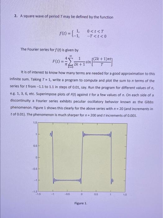
2. A square wave of period 7 may be defined by the function f(0) = { 1 0<t<T -T<t<0 The Fourier series for f (t) is given by 00 1 F(t) == Σ sin in [(2k +1)nt] 2k +11 T k=0 It is of interest to know how many terms are needed for a good approximation to this infinite sum. Taking T = 1, write a program to compute and plot the sum to n terms of the series for t from-1.1 to 1.1 in steps of 0.01, say. Run the program for different values of n, e.g. 1, 3, 6, etc. Superimpose plots of F(t) against t for a few values of n. On each side of a discontinuity a Fourier series exhibits peculiar oscillatory behavior known as the Gibbs phenomenon. Figure 1 shows this clearly for the above series with n = 20 (and increments in t of 0.01). The phenomenon is much sharper for n = 200 and t increments of 0.001. 1.5 0.5- OF -0.5- ME 0 0.5 1.5 Figure 1. -1.5 1.5 -1 -0.5