Answer Happy

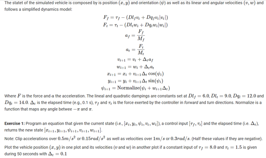
The state of the simulated vehicle is composed by is position (2, y) and orientation () as well as its linear and angular velocities (v, w) and follows a simplified dynamics model: F; = Ti - (DjV; + Davi|vil) Fe = T1 - (D1_w; + Dą.w|wk| Fj aj M ay = F M Vf+1 = 0 + Ata Wi+1 = w; + A, a 21+1 = 8; + 0x+1A, cos(i) Yi+1 = Yi + V4+1 A, sin(3) Pi+1 = Normalize($i + Wi+1A) Where F is the force and a the acceleration. The lineal and quadratic dampings are constants set at Dl; = 6.0, Dų = 9.0, Dq = 12.0 and Dq+ = 14.0. A is the elapsed time (e.g., 0.1 s), Tg and T4 is the force exerted by the controller in forward and turn directions. Normalize is a function that maps any angle betwee – and T. Exercise 1: Program an equation that given the current state (i.e., [Wi, Yi, Vi, Vi, wz]), a control input (Tf, 7+] and the elapsed time (i.e. Ac). returns the new state (x1+1,91+1, Vi+1, Vi+1, W:+1). Note: Clip accelerations over 0.5m/s2 or 0.15rad/s as well as velocities over 1m/s or 0.3rad/s. (Half these values if they are negative). Plot the vehicle position (x, y) in one plot and its velocities (v and w) in another plot if a constant input of Tj = 8.0 and T4 = 1.5 is given during 50 seconds with A, = 0.1