Answer Happy

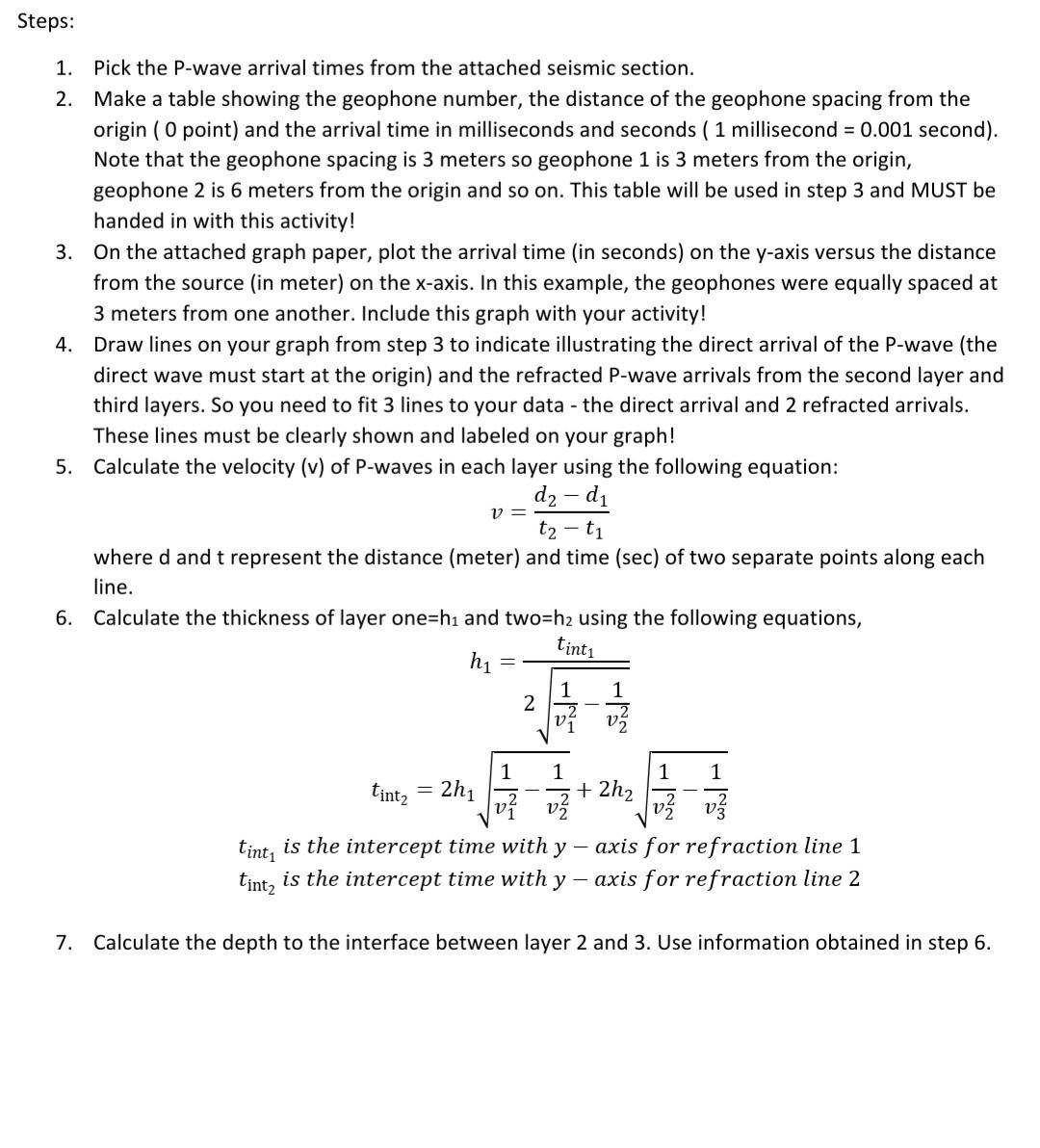
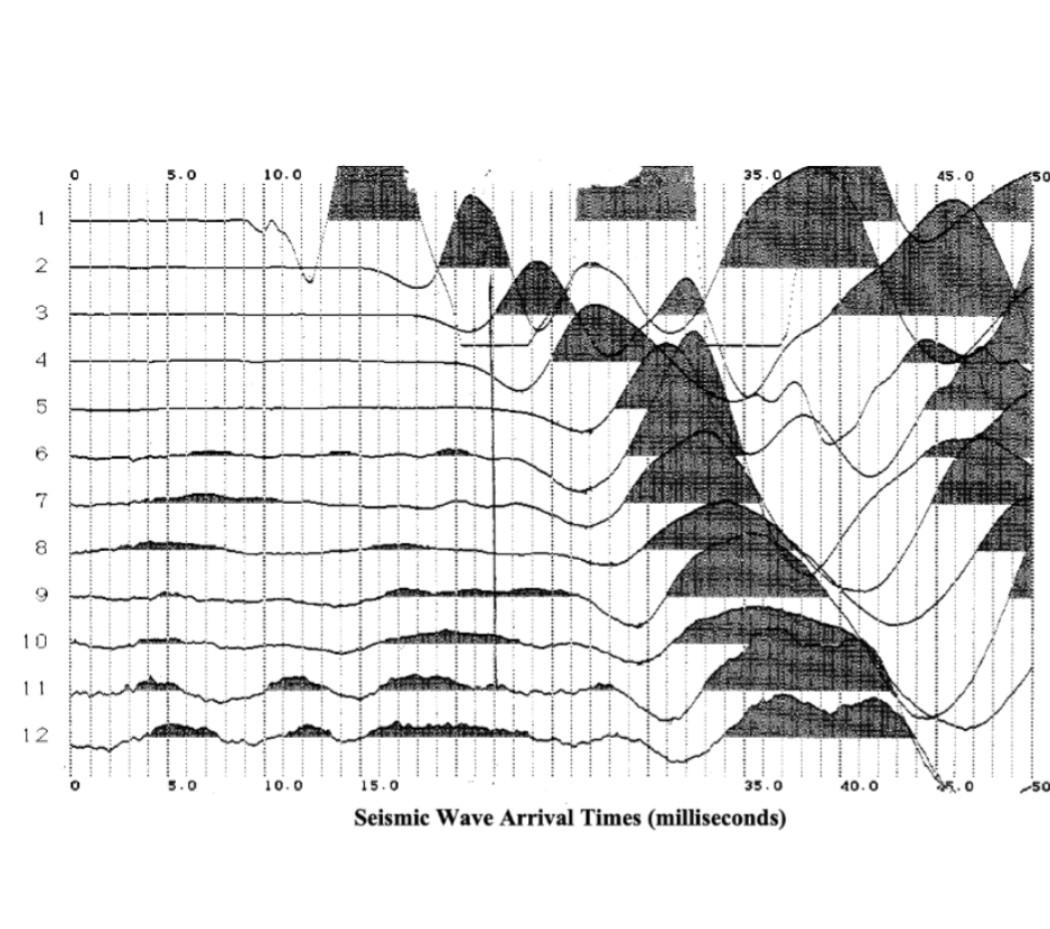
Steps: 1. Pick the P-wave arrival times from the attached seismic section. 2. Make a table showing the geophone number, the distance of the geophone spacing from the origin (O point) and the arrival time in milliseconds and seconds ( 1 millisecond = 0.001 second). Note that the geophone spacing is 3 meters so geophone 1 is 3 meters from the origin, geophone 2 is 6 meters from the origin and so on. This table will be used in step 3 and MUST be handed in with this activity! 3. On the attached graph paper, plot the arrival time in seconds) on the y-axis versus the distance from the source (in meter) on the x-axis. In this example, the geophones were equally spaced at 3 meters from one another. Include this graph with your activity! 4. Draw lines on your graph from step 3 to indicate illustrating the direct arrival of the P-wave (the direct wave must start at the origin) and the refracted P-wave arrivals from the second layer and third layers. So you need to fit 3 lines to your data - the direct arrival and 2 refracted arrivals. These lines must be clearly shown and labeled on your graph! 5. Calculate the velocity (v) of P-waves in each layer using the following equation: dz-d, t2-ti where d and t represent the distance (meter) and time (sec) of two separate points along each line. 6. Calculate the thickness of layer one=hi and two=h2 using the following equations, tinti hi - V= 1 1 2 ví 12 1 1 1 1 tintz va - 2h1 + 2h2 v 7 v2 V3 tint, is the intercept time with y - axis for refraction line 1 tint, is the intercept time with y - axis for refraction line 2 7. Calculate the depth to the interface between layer 2 and 3. Use information obtained in step 6.

5.0 10.0 35.0 45.0 2 3 4 5 6 7 8 9 10 11 12 o 5.0 10.0 15.0 35.0 40.0 50 Seismic Wave Arrival Times (milliseconds)

8. Interpret the composition of each layer using the following table: Material: Typical velocity (meter/sec): Dry soil (vadose zone) 300 Moist soil (vadose zone) 600 – 900 Saturated soil (phreatic zone) ~ 1500 Compact, wet glacial till ~1800 Shale 2100 – 2700 Sandstone 2400 – 3650 Limestone 3650 - 4870 Granite > 5180 9. Draw a soil/rock column showing your interpretation with the thicknesses of units (based on your calculations in steps 7 and 8) and types of soils or rock (based on step 9). Clearly identify the depth of the water table (top of saturated soil).