Answer Happy

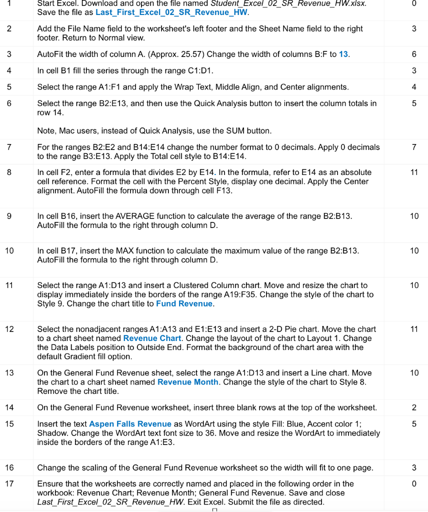
1 0 Start Excel. Download and open the file named Student_Excel_02_SR_Revenue_HW.xlsx. Save the file as Last_First_Excel_02_SR_Revenue_HW. Add the File Name field to the worksheet's left footer and the Sheet Name field to the right footer. Return to Normal view. 2 3 3 6 4 3 AutoFit the width of column A. (Approx. 25.57) Change the width of columns B:F to 13. In cell B1 fill the series through the range C1:01. Select the range A1:F1 and apply the Wrap Text, Middle Align, and Center alignments. Select the range B2:E13, and then use the Quick Analysis button to insert the column totals in row 14. 5 4 6 5 7 7 Note, Mac users, instead of Quick Analysis, use the SUM button. For the ranges B2:E2 and B14:E14 change the number format to 0 decimals. Apply O decimals to the range B3:E13. Apply the Total cell style to B14:E14. In cell F2, enter a formula that divides E2 by E14. In the formula, refer to E14 as an absolute cell reference. Format the cell with the Percent Style, display one decimal. Apply the Center alignment. AutoFill the formula down through cell F13. 8 11 9 10 In cell B16, insert the AVERAGE function to calculate the average of the range B2:B13. AutoFill the formula to the right through column D. 10 10 In cell B17, insert the MAX function to calculate the maximum value of the range B2:B13. AutoFill the formula to the right through column D. 11 10 Select the range A1:D13 and insert a Clustered Column chart. Move and resize the chart to display immediately inside the borders of the range A19:F35. Change the style of the chart to Style 9. Change the chart title to Fund Revenue. 12 11 Select the nonadjacent ranges A1:A13 and E1:E13 and insert a 2-D Pie chart. Move the chart to a chart sheet named Revenue Chart. Change the layout of the chart to Layout 1. Change the Data Labels position to Outside End. Format the background of the chart area with the default Gradient fill option. 13 10 On the General Fund Revenue sheet, select the range A1:D 13 and insert a Line chart. Move the chart to a chart sheet named Revenue Month. Change the style of the chart to Style 8. Remove the chart title. 14 On the General Fund Revenue worksheet, insert three blank rows at the top of the worksheet. 2 15 5 Insert the text Aspen Falls Revenue as WordArt using the style Fill: Blue, Accent color 1; Shadow. Change the WordArt text font size to 36. Move and resize the WordArt to immediately inside the borders of the range A1:E3. 16 3 17 Change the scaling of the General Fund Revenue worksheet so the width will fit to one page. Ensure that the worksheets are correctly named and placed in the following order in the workbook: Revenue Chart; Revenue Month; General Fund Revenue. Save and close Last_First_Excel_02_SR_Revenue_HW. Exit Excel. Submit the file as directed. 0

A B C D E F N WN Aspen Falls Revenue Revenue 4 5 Property Taxes 6 VLF Swap 7 Sales Taxes 8 Other Taxes 9 Vehicle Fees 10 Fines 11 Interest 12 Franchise Fees 13 Development Fees 14 Reimbursements 15 Other Revenue 16 Transfers 17 Total Monthly Revenue January February March 1st Quarter $ 335,039 $ 395,490 S 414,138 $ 1,144,668 383,563 321,421 407,846 1,112,830 408,211 462,010 300,613 1,170,835 118,206 107,461 139,699 365,366 128,227 125,661 133,359 387,246 163,580 157,800 175,140 496,521 168,708 153,371 199,381 521,459 80,455 85,868 89,628 255,951 261,235 237,486 308733 807,455 107735 97,941 127,323 332,998 310,094 354,631 371,020 1,035,744 261,547 237,771 309,102 808,420 $ 2,726,600 $ 2,736,910 $ 2,975,982 $ 8,439,492 Percent of Revenue 13.6% 13.2% 13.9% 4.3% 4.6% 5.9% 6.2% 3.0% 9.6% 3.9% 12.3% 9.6% $ 19 Average Monthly Revenue 20 Maximum Monthly Revenue 227,217 $ 408,211 $ 228,076 $ 462,010 $ 247,998 414,138 $ FUND REVENUE 98888898X8 NSXXNSo ū a 22 23 24 25 26 27 28 29 30 $500,000 $450,000 $400,000 $350,000 $300,000 $250,000 $200,000 $150,000 $100,000 $50,000 Fines VLF Swap interest Sales Tres Transfers Other Taxes Vehicle Fees Property Taxes Franchise Fees 33 34 35 36 37 Other Revenue Reimbursements Development Fees January February March