Page 1 of 1
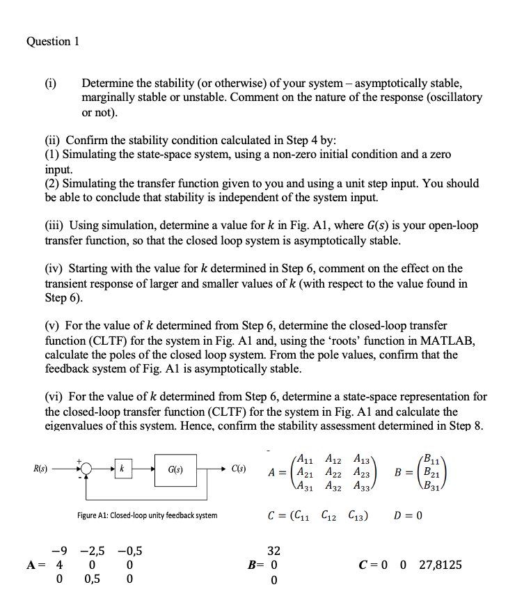
Question 1 (1) Determine the stability (or otherwise) of your system – asymptotically stable, marginally stable or unsta
Posted: Mon May 09, 2022 8:03 am
by answerhappygod
- Question 1 1 Determine The Stability Or Otherwise Of Your System Asymptotically Stable Marginally Stable Or Unsta 1 (121.92 KiB) Viewed 42 times
Question 1 (1) Determine the stability (or otherwise) of your system – asymptotically stable, marginally stable or unstable. Comment on the nature of the response (oscillatory or not). (ii) Confirm the stability condition calculated in Step 4 by: (1) Simulating the state-space system, using a non-zero initial condition and a zero input. (2) Simulating the transfer function given to you and using a unit step input. You should be able to conclude that stability is independent of the system input. (iii) Using simulation, determine a value for k in Fig. Al, where G(s) is your open-loop transfer function, so that the closed loop system is asymptotically stable. (iv) Starting with the value for k determined in Step 6, comment on the effect on the transient response of larger and smaller values of k (with respect to the value found in Step 6). (v) For the value of k determined from Step 6, determine the closed-loop transfer function (CLTF) for the system in Fig. Al and, using the “roots' function in MATLAB, calculate the poles of the closed loop system. From the pole values, confirm that the feedback system of Fig. Al is asymptotically stable. (vi) For the value of k determined from Step 6, determine a state-space representation for the closed-loop transfer function (CLTF) for the system in Fig. Al and calculate the eigenvalues of this system. Hence, confirm the stability assessment determined in Step 8. BU R(s) k G(s) C(s) A11 A12 A13 A = 421 422 423 \A3 A32 A33 B = (B21 B31 Figure A1: Closed-loop unity feedback system C = C11 C12 (13) D=0 -9 A= 4 0 -2,5 -0,5 0 0,5 00 32 B= 0 0 C=0 0 27,8125