Answer Happy

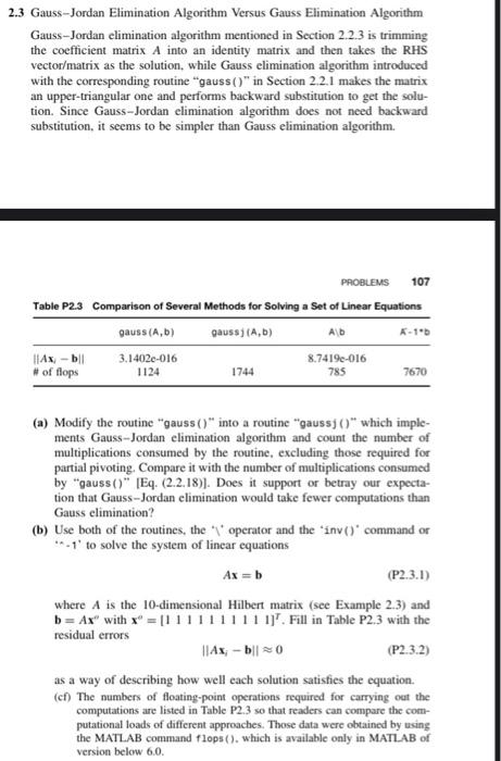
2.3 Gauss-Jordan Elimination Algorithm Versus Gauss Elimination Algorithm Gauss-Jordan elimination algorithm mentioned in Section 2.2.3 is trimming the coefficient matrix A into an identity matrix and then takes the RHS vector/matrix as the solution, while Gauss elimination algorithm introduced with the corresponding routine "gauss()" in Section 2.2.1 makes the matrix an upper-triangular one and performs backward substitution to get the solu- tion. Since Gauss-Jordan elimination algorithm does not need backward substitution, it seems to be simpler than Gauss elimination algorithm. PROBLEMS 107 Table P2.3 Comparison of Several Methods for Solving a Set of Linear Equations gauss (A,b) gaussj (A,b) A\b A-1'b 3.14020-016 ||Ax-b|| # of flops 8.7419e-016 785 1124 1744 7670 (a) Modify the routine "gauss()" into a routine "gaussj ()" which imple- ments Gauss-Jordan elimination algorithm and count the number of multiplications consumed by the routine, excluding those required for partial pivoting. Compare it with the number of multiplications consumed by "gauss()" [Eq. (2.2.18)]. Does it support or betray our expecta- tion that Gauss-Jordan elimination would take fewer computations than Gauss elimination? (b) Use both of the routines, the operator and the inv()' command or **-1' to solve the system of linear equations Ax = b (P2.3.1) where A is the 10-dimensional Hilbert matrix (see Example 2.3) and b= Ax" with x = [1 1 1 1 1 1 1 1 1 1]. Fill in Table P2.3 with the residual errors ||Ax-b|| 0 (P2.3.2) as a way of describing how well each solution satisfies the equation. (cf) The numbers of floating-point operations required for carrying out the computations are listed in Table P2.3 so that readers can compare the com- putational loads of different approaches. Those data were obtained by using the MATLAB command flops (). which is available only in MATLAB of version below 6.0.