- Solution First Let Us Consider What Information Can Be Obtained Directly From The Differential Equation Itself Suppose 1 (101.66 KiB) Viewed 43 times
- Solution First Let Us Consider What Information Can Be Obtained Directly From The Differential Equation Itself Suppose 2 (28.44 KiB) Viewed 43 times

- Solution First Let Us Consider What Information Can Be Obtained Directly From The Differential Equation Itself Suppose 3 (25.19 KiB) Viewed 43 times
draw direction fields ro describe the damiku solitions
- Solution First Let Us Consider What Information Can Be Obtained Directly From The Differential Equation Itself Suppose 4 (25.19 KiB) Viewed 43 times
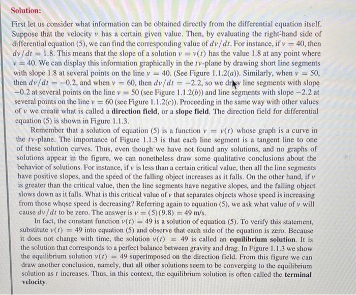
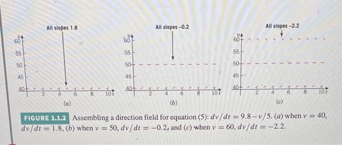
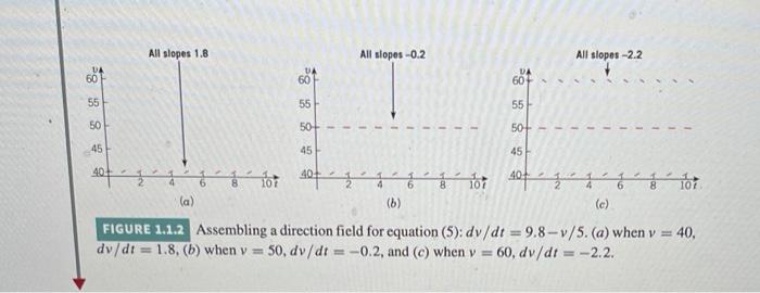
Solution: First let us consider what information can be obtained directly from the differential equation itself. Suppose that the velocity v has a certain given value. Then, by evaluating the right-hand side of differential equation (5), we can find the corresponding value of dv/dt. For instance, if v = 40, then dv/dt = 1.8. This means that the slope of a solution v = v(t) has the value 1.8 at any point where v = 40. We can display this information graphically in the tv-plane by drawing short line segments with slope 1.8 at several points on the line v = 40. (See Figure 1.1.2(a)). Similarly, when v = 50, then dv/dt = -0.2, and when v = 60, then dv/dt = -2.2, so we dry line segments with slope -0.2 at several points on the line v = 50 (see Figure 1.1.2(b)) and line segments with slope -2.2 at several points on the line v = 60 (see Figure 1.1.2(c)). Proceeding in the same way with other values of v we create what is called a direction field, or a slope field. The direction field for differential equation (5) is shown in Figure 1.1.3. Remember that a solution of equation (5) is a function v = v(1) whose graph is a curve in the tv-plane. The importance of Figure 1.1.3 is that each line segment is a tangent line to one of these solution curves. Thus, even though we have not found any
solutions, and no graphs of
solutions appear in the figure, we can nonetheless draw some qualitative conclusions about the behavior of
solutions. For instance, if v is less than a certain critical value, then all the line segments have positive slopes, and the speed of the falling object increases as it falls. On the other hand, if v is greater than the critical value, then the line segments have negative slopes, and the falling object slows down as it falls. What is this critical value of v that separates objects whose speed is increasing from those whose speed is decreasing? Referring again to equation (5), we ask what value of v will cause dv/dt to be zero. The answer is v = (5)(9.8) = 49 m/s. In fact, the constant function v(t) = 49 is a solution of equation (5). To verify this
statement, substitute (1) 49 into equation (5) and observe that each side of the equation is zero. Because it does not change with time, the solution (1) = 49 is called an equilibrium solution. It is the solution that corresponds to a perfect balance between gravity and drag. In Figure 1.1.3 we show the equilibrium solution v(1) = 49 superimposed on the direction field. From this figure we can draw another conclusion, namely, that all other
solutions seem to be converging to the equilibrium solution as t increases. Thus, in this context, the equilibrium solution is often called the terminal velocity
All slopes 1,8 All slopes -0.2 All slopes -2.2 VA 60 60 601 55 55 55 50 50- 50 45 45 45 10 40 40+ 2. 1 o 8 - 10 not 401 2 2 4 8 107 6 107 6 8 (a) (6) (c) FIGURE 1.1.2 Assembling a direction field for equation (5): dv/dt = 9.8-v/5. (a) when v = = 40, dv/dt = 1.8, (b) when v = 50, dv/dt = -0.2, and (c) when v = 60, dv/dt = -2.2.
All slopes 1.8 All slopes -0.2 All slopes -2.2 VA 60 UA 60 VA 60+ 55 55 55 50 50+ - 50+ 45 45 45 402 of aggior not at a loi notri 6 8 10 la) (6) (e) FIGURE 1.1.2 Assembling a direction field for equation (5): dv/dt = 9.8-v/5. (a) when v = 40, dv/dt = 1.8. (b) when v = 50, dv/dt = -0.2, and (c) when y = 60, dv/dt = -2.2.