MATLAB
Please help me out walk through this. It needs MATLAB work.
Thank you all for your time.
MATLAB
- Matlab Please Help Me Out Walk Through This It Needs Matlab Work Thank You All For Your Time Matlab 1 (218.58 KiB) Viewed 20 times
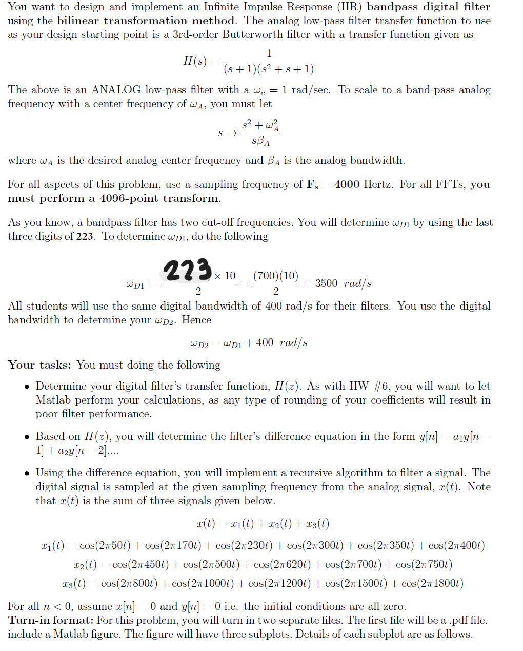
You want to design and implement an Infinite Impulse Response (IIR) bandpass digital filter using the bilinear transformation method. The analog low-pass filter transfer function to use as your design starting point is a 3rd-order Butterworth filter with a transfer function given as 1 (s + 1)(52 + s +1) The above is an ANALOG low-pass filter with a we = 1 rad/sec. To scale to a band-pass analog frequency with a center frequency of WA, you must let HS) = 6/s ² + w? S → SBA where wa is the desired analog center frequency and BA is the analog bandwidth. For all aspects of this problem, use a sampling frequency of Fs = 4000 Hertz. For all FFTs, you must perform a 4096-point transform. As you know, a bandpass filter has two cut-off frequencies. You will determine wpi by using the last three digits of 223. To determine wpi, do the following 223 x 10 (700)(10) WD1 = = 3500 rad/s 2 2 All students will use the same digital bandwidth of 400 rad/s for their filters. You use the digital bandwidth to determine your wp2. Hence WD2 = wp1 + 400 rad/s Your tasks: You must doing the following • Determine your digital filter's transfer function, H(2). As with HW #6, you will want to let Matlab perform your calculations, as any type of rounding of your coefficients will result in poor filter performance. • Based on H(z), you will determine the filter's difference equation in the form y[n] = a1y[n – 1] +azy[n – 2.... • Using the difference equation, you will implement a recursive algorithm to filter a signal. The digital signal is sampled at the given sampling frequency from the analog signal, r(t). Note that r(t) is the sum of three signals given below. r(t) = x1(t) + x2(t) + x3(t) 21(t) = cos(250t) + cos(26170t) + cos(2T230t) + cos(27300t) + cos(27350t) + cos(27400t) X2(t) = cos(26450t) + cos(27500t) + cos(27620t) + cos(21700t) + cos(21750t) 13(t) = cos(27800t) + cos(211000t) + cos(271200t) + cos(271500t) + cos(271800t) For all n < 0, assume x[n] = 0 and y[n] = 0 i.e. the initial conditions are all zero. Turn-in format: For this problem, you will turn in two separate files. The first file will be a .pdf file. include a Matlab figure. The figure will have three subplots. Details of each subplot are as follows. = = =
• The first subplot, subplot(3,1,1), will be a plot of the magnitude of the frequency response of your filter, (H(-)). The x-axis will be a semilog axis and the units will be in Hertz. The limits will be from 1 Hz to 2 kHz. The y-axis will be in dB, and will run from -100 dB to +5 dB. For many of your filters, the stop band of your filter will be less than -100 dB; this is fine. The passband gain for all of your filters will be 0 dB. • The second subplot, subplot(3,1,2), will be a plot of the magnitude of the 4096-point FFT of X(t). When you plot the magnitude, be sure to scale the magnitude by N/2 (i.e. 2048). The X-axis will be linear and the units will be in Hertz. The x-axis will range from 0 Hz to 2 kHz. Recall, when plotting the FFT values, use stem. The y-axis will have limits from 0 to 1.5. • The third subplot, subplot(3,1,3), will be a plot of the magnitude of the 4096-point FFT of y(t), where y(t) is the output of your filter (i.e. the result of your recursive algorithm). When you plot the magnitude, be sure to scale the magnitude by N/2 (i.e. 2048). The x-axis will be linear and the units will be in Hertz. The x-axis will range from 0 Hz to 2 kHz. Recall, when plotting the FFT values, use stem. The y-axis will have limits from 0 to 1.